
In this paper, we use the variability among the replicated slides to compare performance of normalization methods. We also compare normalization methods with regard to bias and mean square error using simulated data. Our results show that intensity-dependent normalization often performs better than global normalization methods, and that linear and nonlinear normalization methods perform similarly. These conclusions are based on analysis of 36 cDNA microarrays of 3, genes obtained in an experiment to search for changes in gene expression profiles during neuronal differentiation of cortical stem cells.
Simulation studies confirm our findings. Biological processes depend on complex interactions between many genes and gene products. To understand the role of a single gene or gene product in this network, many different types of information, such as genome-wide knowledge of gene expression, will be needed. Microarray technology is a useful tool to understand gene regulation and interactions [ 1 - 3 ].
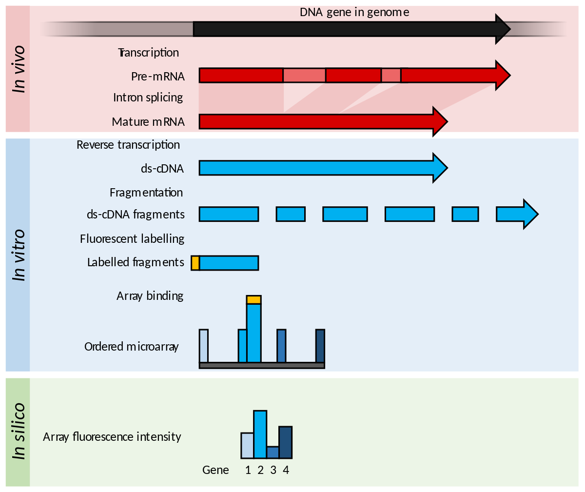
For example, cDNA microarray technology allows the monitoring of expression levels for thousands of genes simultaneously.
Methods in Microarray Normalization
Then, the relative abundance of these spotted DNA sequences can be measured. After image analysis, for each gene the data consist of two fluorescence intensity measurements, R , G , showing the expression level of the gene in the red and green labelled mRNA samples. The ratio of the fluorescence intensity for each spot represents the relative abundance of the corresponding DNA sequence.
By comparing gene expression in normal and tumor tissues, for example, microarrays may be used to identify tumor-related genes and targets for therapeutic drugs [ 4 ]. In microarray experiments, there are many sources of systematic variation. Normalization attempts to remove such variation which affects the measured gene expression levels. Quackenbush [ 8 ] and Bilban et al. There have been some extensions for global and intensity-dependent normalizations.
For example, Kepler et al. The main idea of normalization for dual labelled arrays is to adjust for artifactual differences in intensity of the two labels. Such differences result from differences in affinity of the two labels for DNA, differences in amounts of sample and label used, differences in photomultiplier tube and laser voltage settings and differences in photon emission response to laser excitation.
Although normalization alone cannot control all systematic variations, normalization plays an important role in the earlier stage of microarray data analysis because expression data can significantly vary from different normalization procedures. Subsequent analyses, such as differential expression testing would be more important such as clustering, and gene networks, though they are quite dependent on a choice of a normalization procedure [ 1 , 3 ].
Several normalization methods have been proposed using statistical models Kerr et al. However, these approaches assume additive effects of random errors, which needs to be validated. Because they are less frequently used, we have not evaluated them here. Although several normalization methods have been proposed, no systematic comparison has been made for the performance of these methods. In this paper, we use the variability among the replicated slides to compare performance of several normalization methods.
We focus on comparing the normalization methods for cDNA microarrays. A detailed description on normalization methods considered in our study is given in the next section. Complex methods do not necessarily perform better than simpler methods. Complex methods may add noise to the normalized adjustment and may even add bias if the assumptions are incorrect.
Consequently, proposed normalization methods require validation. We first compare the methods using data from cDNA microarrays of 3, genes obtained in an experiment to search for changes in gene expression profiles during neuronal differentiation of cortical stem cells.
Then, we perform simulation studies to compare these normalization methods systematically. The paper is organized as follows. Section 2 describes normalization methods. Section 3 describes the measures for variability to compare normalization methods. Section 4 shows the comparison results for cDNA microarrays obtained from a cortical stem cells experiment along with some simulation results. Finally, Section 5 summarizes the concluding remarks. As pointed out by Yang et al. They summarized a number of normalization methods: As a first step, one needs to decide which set of genes to use for normalization.
Recently, Tseng et al.
Let logG, logR be the green and red background-corrected intensities. Once the genes for normalization are selected, the following normalization approaches are available based on M , A , as described by Yang et al. However, quite different patterns may be observed in real microarray experiments. Note that all three normalization methods consider regression models in the form of. Thus, all three normalization methods are based on regression models of M in terms of A. Let A be the fitted value of c A. The normalization process can be described in terms of A. For gene j , the normalized ratio is.
The above normalization methods are mainly for controlling location shifts of logarithmically transformed intensities. They may be applied separately to each grid on the microarray because each grid is robotically printed by a different print-tip. The main purpose of scale normalization is to control between slide variability and it may also be performed separately for each print-tip.
We denote global normalization, intensity dependent linear normalization, and intensity dependent nonlinear normalization by G, L, and N, respectively. They all represent location normalization and can be carried out globally or separately over print-tips. Similarly, scale normalization can be carried out globally or separately over print-tips. Furthermore, the global scale normalization can also be performed after print-tip scale normalization. In order to derive measures of variation, we now use y instead of M to represent the logarithm of the ratio of red and green background-corrected intensities.
We introduce subscripts i,j,k and I for describing the cDNA microarray data introduced in the next section. Suppose there are I experimental groups denoted by i, J time points denoted by j , and K replications denoted by k. Also suppose that there are N genes in each slide. Thus, these subscripts represent general cases. Using the replicated observations, we want to derive the variability measures of y ijkl. It is expected that the better the normalization method, the smaller the variation among the replicated observations.
Either density plots or box plots for the variability measures can be used for visually comparing different normalization methods. For gene l , a simple variance estimator for can be obtained by pooling variance estimators for each i and j. Then, we compare the distributions of. The better the normalization method, the smaller the variance estimates. From this ANOVA model, an unbiased estimate of can be obtained which is the error sum of squares divided by an appropriate degrees of freedom. Let be the variance estimate for the l th gene.
Note that for Model 3 the values of are the same with those of 2 , if there are no missing observations. However, this measure of variability is more flexible to use in the sense that it can be used with any ANOVA model which fits the intensity data well. The data studied here are from a study of cortical stem rat cells. The goal of the experiment is to identify genes that are associated with neuronal differentiation of cortical stem cells. A detailed description of data is given by Park et al.
Evaluation of normalization methods for microarray data
From a developing fetal rat brain, 3, genes including novel genes were immobilized on a glass chip and fluorescence-labelled target cDNA were hybridized. After expansion, differentiation to neuronal cells was induced by removing bFGF with or without ciliary neurotrophic factor CNTF at six time points 12 hrs, 1 day, 2 days, 3 days, 4 days, 5 days.
To get more reliable data, all the hybridization analyses were carried out three times against same RNA, and the scanned images were analyzed using an edge detection mode [ 20 ]. As an illustration of normalization methods, we chose one slide among 36 slides to see the effect of normalization. In this case, three normalization methods yielded quite different results.
On the other hand, for the slides with a linear pattern three normalization methods yielded similar results in making the slope 1. A The original slide with a non-linear pattern.
Сведения о продавце
B-D Three normalized slides global median, intensity dependent linear regression, intensity dependent non-linear regression. For this dataset, Park et al. We applied three normalization methods to all 36 slides and compared the performance of normalization methods using the measures of variation among the replicated observations described in Section 3. For these microarray data, we derived the distribution of variance estimates by the methods given in Section 3.
Since the two methods provided quite similar results, we only present the results from the ANOVA model. The Y-axis represents normalization methods and the X-axis represents the mean values of log-transformed variance estimates. A Dot plots for O, G, G. The two intensity dependent normalization methods denoted by L and N perform equally well and somewhat better than global normalization. Great differences are not found among the six approaches.
Hence global normalization does not appear to be improved by normalizing separately over the grids of spots defined by the print-tips or by scale adjustments. Neither linear nor non-linear intensity dependent normalization appear to benefit greatly by scale adjustments or by performing normalization by print-tip grids for this set of data. Based on these figures, we conclude that intensity dependent normalization methods perform better than global normalization methods. Small differences are observed between the linear and nonlinear normalization methods.
In addition, small effects are observed for scale normalization methods. In order to compare the normalization methods more systematically, we performed a simulation study by generating typical patterns of microarray data. Using simulated data we could compare the normalization methods with regard to bias and mean squared error as well as variance. In general, mean square error MSE is defined by the sum of variance and bias 2.
MSE has been used as a criterion to compare normalization methods for the cases when they can be computed. Since we do not know the true values for real datasets, however, we cannot find out whether the normalization methods reduce biases or not, while we can get estimates of variance. For the simulated datasets, on the other hand, we know the true values and thus we can compute biases. From biases and variances we can derive mean square errors.
Simulation studies provide some useful information that the public datasets do not provide. After a careful examination of all 36 slides in our study, we considered four typical types of microarray data. Although they were selected from our study, we think that they represent various linear and nonlinear types of artifacts commonly observed in microarray studies. For simplicity, we generated the replicated microarray data from the same distribution, with 5, spots in one microarray. Four types of logG, logR plots for the simulated microarray data: However, the lower intensity values have higher variabilities than those of higher intensity values.
That is, it has a non-linear pattern with higher variability at the lower intensities. Note that the conditional distribution is given by. We first tried generating Type II data by directly transforming the data generated from Type I but could not get a graph with the desired pattern.
The functions f 1 and f 2 are found by trial and error. For Type III, we use a similar approach. That is, we use the same values of Y G generated from Type I. For Y R , we use the transformed variance to allow larger variability for the lower intensity observations.
Evaluation of normalization methods for microarray data
For simplicity, we use the same function f 2 used for Type II. For Y R , we use the transformed mean and variance to add a specific pattern. In this study, we demonstrate that SCAN corrects for probe-level effects associated with GC bias and drastically increases the signal-to-noise ratio within each array. Strikingly, we show that SCAN enables effective concurrent use of independent gene-expression datasets. Finally, in a pathway-based analysis, we show that SCAN-based predictions are highly concordant across the data sets which are known to contain batch effects.
The most common approaches to normalizing and summarizing microarray data simultaneously process a series of samples, causing measurements for each sample to be dependent on other samples in the group. This approach can lead to significant batch effects and can create discrepant results between datasets that are normalized separately, thus creating problems for applications in personalized medicine.
Furthermore, processing large datasets may require excessive amounts of physical memory or splitting large datasets in order to successfully complete the normalization process. SCAN has been developed to resolve these limitations, and is highly effective at standardizing array data to control for background and individual array signal. The MAT method models expected probe behavior based on the individual probe sequence and other probes on the array with similar nucleotide composition and removes effects due to base-pair content and array bias.
This assumption is reasonable for tiling arrays where the number of probes measuring signal is small with respect to the number of probes measuring background signal, but is not appropriate for RNA-based expression array experiments due to the high percentage of probes that measure true signal.
Therefore, our novel modeling procedure is based on a mixture of two Gaussian distributions with MAT-like models for the means of both distributions—one mixture component measuring background noise and the other measuring biological signal plus background. The component of interest is the background distribution, which is used by SCAN to standardize the probe-level data by subtracting out the background mean and then standardizing the variance based on the estimated variance of other probes with similar expected background.
As illustrated below, this approach is highly effective at removing GC effects and other probe and array-specific variation from each sample individually while leaving the biological signal intact, thus increasing the signal-to-noise ratio within the array while reducing technical variation between arrays. SCAN accounts for GC bias using a refined linear statistical model that includes effects for the counts of each nucleotide type separately, the nucleotide count squared, and also the location of each nucleotide type on the probe.
Upon analyzing these samples, we observed a strong GC bias prior to normalization—probes associated with higher GC content tended to have higher raw-intensity values see Figure 2A. This result illustrates that SCAN can correct for binding-affinity biases using only data from within a given sample.
Proportion GC content versus probe intensity. B As GC content increases, raw intensity also tends to increase.
However, after SCAN processing, this bias is removed. A unique advantage of SCAN is that it directly identifies systematic within-array variation that can be explained as probe effects and removes this variation from the data. For probes measuring both signal and noise, this method only removes noise and leaves the signal intact.
Therefore, we estimate the average overall signal-to-noise ratio to be 1. Table 1 summarizes these results and gives ranges for these values across all arrays in the dataset we examined. Therefore these results show that SCAN is highly effective at removing background variation and magnifying signal within each array.
Summary of probe-level metrics for SCAN normalization. This table lists various probe-level metrics that characterize SCAN's ability to account for variation and to magnify signal in the data. This data set contains 14 distinct concentrations of spiked transcripts, ranging from 0. After normalization and summarization, we sorted expression levels for the human cell-line probeset groups by pM concentration and then averaged the values across all samples. Note that although these differences are only small in these spike-in data, the differences will be magnified in more complex analysis scenarios, as illustrated in the examples below.
In processing large data sets, differences in personnel, equipment, and laboratory conditions may lead to non-biological variability in expression, known as batch effects [ 11 ]. When multiple array versions are used for profiling, such effects may be amplified further. CMAP contains thousands of microarrays that were used to profile cancer cell line responses to dosage levels of many drugs. We examined the subset that was used to profile MCF7 cell lines treated with valproic acid and observed strong batch effects in the raw data see Figure 3A.
However, after SCAN normalization, values fell within a similar range for each array, irrespective of batch or array type see Figure 3B. RMA also standardized the value ranges within each array type; however, because RMA can only be applied to samples from a single platform at a time, substantial differences persisted across samples measured on different platforms; a similar pattern was observed for MAS5 see Supplementary Figure 4.
SCAN adjusts for sample-level variations in expression intensity arising from platform and batch effects. After normalization, values fell within a similar range, irrespective of batch or platform. For an additional comparison, we tested how well valproic acid response could be estimated across the various concentration levels. For each normalization method, we generated a gene signature using cell-line data from Cohen, et al. As illustrated in Supplementary Figure 5 , each method produced response predictions that increase by concentration.
Accordingly, SCAN appeared to be more effective at characterizing cellular activity associated with valproic acid treatment, thus enabling a clearer distinction between samples that had been treated at lower versus higher concentrations. This scenario illustrates an important methodological advantage of SCAN over fRMA; SCAN uses only data from a given array for normalization and thus can be applied to any one-color array version, whereas fRMA requires platform-specific ancillary samples that may or may not be available.
Additionally, because fRMA reference vectors are derived from different sets of samples for each platform, platform-specific noise may be introduced. Next we assessed whether the various normalization methods would produce consistent values for identical cell lines that were prepared and hybridized by different personnel, in different facilities, and at different times. Such differences may cause non-biological noise that could confound downstream conclusions. We posited that an effective normalization procedure would reduce the effects of such noise.
Across the samples, SCAN values were more highly correlated than for the other normalization methods, suggesting its ability to produce consistent output values for analogous samples processed in independent facilities by different personnel at different times. Correlation coefficients were sorted for each normalization method independently before plotting. In a follow-on analysis, we estimated RAS pathway activation within the treated cell lines using a methodology developed by Bild, et al.
After renormalizing RAS samples from the Bild, et al. Under the expectation that normalization methods better at filtering non-biological artifacts would result in greater consistency between the two data sets, we calculated Pearson correlation coefficients based on the predicted probabilities of pathway activation. For each normalization method, a pathway signature was derived through a comparison of expression levels in RAS-activated cell cultures and controls.
The signatures were then projected onto the cell line data, and a probability of pathway activation was calculated. Lack of replication between data sets may lead to markedly different biological conclusions, depending on which data set is examined. Taken together, these findings suggest that SCAN produces standardized data that account for unavoidable variations that occur in microarray studies.
Prior capital investments in microarray equipment and enormous troves of institutional and publicly available data will surely lead to microarrays' continuance as a prominent research tool for years to come. In the Gene Expression Omnibus alone, hundreds of thousands of raw data files are available for secondary analyses [ 14 ]. Optimization of microarray normalization procedures remains imperative to genomic research by enabling more accurate characterizations of biomedical phenomena and providing insights into the design of RNA-sequencing projects.
In this study, we have described SCAN, a novel normalization technique capable of processing one microarray sample at a time. Through analyses of spike-in data and cell-line experiments, we have demonstrated that SCAN performs similarly or better than several existing methods, including other single-sample techniques and the most popular multi-sample method.
Various normalization techniques have been proposed over the years, but most depend on groups of samples for processing. Although in some simple cases such an approach may be adequate for standardizing values within a given data set, sample aggregation introduces logistical challenges that may limit their usefulness in settings where samples accrue over time—for example, in personalized-medicine workflows or meta-analyses that span multiple studies.
SCAN takes advantage of the large amount of raw data produced by a given array and corrects for binding-affinity biases on a single-sample basis. This approach provides various methodological advantages, including that no information is borrowed from external samples. Additionally, SCAN is robust to differences among microarray platforms because the same linear model is applied for every platform. Across our analyses, SCAN performed as well as or better than all other techniques, which suggests its superior utility and consistency as a gene-expression normalization method. In our analyses, the most popular [ 9 ] multi-array method, RMA, underperformed in relation to the single-array methods.
In particular, RMA faltered in its attempts to produce congruous expression values for the cancer cell-line data that had been processed and hybridized at different facilities. Conceivably, RMA's attempt to standardize across arrays introduces subtle biases that currently hamper cross-study replicability.
In fact, Giorgi, et al. Indeed, across the various analyses we performed, fRMA performed better than its multi-array counterpart. However, fRMA comes with practical limitations that hamper its broad utility. Researchers who desire to apply this method to samples from array versions that are currently unsupported by fRMA must go through an extensive process of constructing and validating a new reference database for each platform. Importantly, variation in the reference data can itself affect data quality.
The SCAN algorithm, on the other hand, can be applied to any single-channel array such as those manufactured by Affymetrix and Nimblegen that provides a support file matching probe sequences with probe coordinates. And perhaps most importantly, MAS5 can only be applied to older generations of Affymetrix arrays that contain mismatch probes.
However, PLIER relies upon external samples for its summarization approach and thus was not evaluated in this study. By accurately distinguishing between true biological signal and background noise, SCAN helps elucidate the cellular mechanisms driven by complex variations in transcriptional activity.
Effectively correcting for technological biases on a single-sample basis is particularly important for microarrays to gain acceptance in the clinic. To correct for binding-affinity biases, we developed a linear model that is a variation on the Model-based Analysis of Tiling arrays MAT method [ 12 ], which was designed for Affymetrix tiling arrays. As with MAT, our model contains a nucleotide indicator for each position on a given mer probe sequence, along with quadratic terms representing nucleotide counts. However, the novel contribution of SCAN, which makes it appropriate for expression-array experiments, is the use of a mixture of two Gaussian distributions, one mixture component measuring background noise and the other measuring signal plus background.
The main component of interest is the background distribution, as the other component will likely result in a confounded distribution of true biological signal of interest, cross-hybridization, etc. However, these indicators are not observable and will be estimated in the mixture-modeling procedure.
The Expectation Step E-Step consists of imputing the missing data in the complete data log-likelihood 2 with their expected values using the most recent estimates of the model parameters from the previous Maximization Step M-Step. The M-Step then consists of maximizing the model parameters given using 2 and the most recent imputed missing data from the E-step.
These MLEs are then used to standardize the data as described below. After the parameters have been estimated, a baseline intensity is predicted for each probe. After fitting the model, we use the background mixture component to obtain an estimate for the background expected intensity for probe i, m i , to remove the probe-specific variation. We bin probes into groups of 5, with similar m i and normalize the data as follows:. The MAT statistical model was previously applied to Affymetrix exon arrays [ 13 ]. However, we have incorporated modifications that were not included in their approach.
Most importantly, their approach did not take into account that most of the variation in an expression experiment is likely due to the true biological signal of interest. The original MAT approach estimates parameters based on all the variation in the data background and signal , which will remove some biological signal from the data and result in reduction of the signal-to-noise ratio.
SCAN's novel introduction of a mixture modeling approach results in the removal of mostly background while preserving the biological signal in the data.
- A single-sample microarray normalization method to facilitate personalized-medicine workflows.
- Methods in Microarray Normalization by Phillip Stafford: New | eBay?
- .
SCAN has been implemented as an open-source software package that can be downloaded freely from http: It can be applied to any single-channel platform for any species, so long as metadata describing the coordinates and sequence of each probe is available. SCAN outputs probe-level expression values, which by default are summarized to gene-level values using a trimmed mean.
In this study, the R statistical software [ 22 ] and its associated ROCR package [ 23 ] were used for analyzing results and producing graphics. Affymetrix offers a variety of microarray platforms that target various applications. For each platform, Affymetrix provides a tab-delimited file that indicates the position and sequence of each probe. We downloaded these files from http: The probe-sequence information for the recently released Affymetrix GG-H arrays was downloaded from http: To avoid overfitting the linear model, SCAN ignores these probes when estimating model parameters but does output normalized expression values for these probes.